Introduction
Exploratory Factor Analysis (EFA) is a powerful multivariate statistical technique used to uncover the latent structure underlying a set of observed variables. In biological and health sciences, EFA is particularly useful in analyzing physiological measurements to identify hidden constructs that explain correlations among variables. This article walks you through a complete EFA workflow in R using physiological data, including code, interpretation, visualizations, and best practices.
What is Exploratory Factor Analysis (EFA)?
EFA aims to reduce a large number of observed variables into a smaller set of unobserved factors. Unlike Principal Component Analysis (PCA), which is purely a data reduction technique, EFA models the underlying latent constructs believed to influence the measured variables.
Why Use EFA in Biological Sciences?
Biological data often include interrelated physiological variables (e.g., blood pressure, cholesterol, glucose). EFA helps uncover the underlying health domains such as cardiovascular health or metabolic function that affect these variables.
Required Packages in R
Install and load the required packages:
install.packages("psych") # For factor analysis functions
install.packages("GPArotation") # For rotation methods
library(psych)
library(GPArotation)
Preparing the Dataset
In this tutorial, we use a synthetic dataset representing 20 individuals and their physiological measurements:
physio_data <- data.frame(
Systolic_BP = c(122,135,118,140,130,125,138,120,145,132,117,129,142,121,133,126,139,119,136,124),
Diastolic_BP = c(78,88,76,92,85,82,90,79,95,87,74,84,93,80,86,83,91,77,89,81),
Glucose = c(95,110,90,115,102,98,108,94,120,105,88,100,118,96,107,99,113,92,112,97),
Cholesterol = c(180,200,170,210,195,185,205,175,215,190,165,188,212,178,198,182,208,172,202,183),
BMI = c(24.3,27.1,22.5,29.3,25.0,23.8,28.0,24.0,30.5,26.3,21.9,25.5,29.8,23.5,26.0,24.6,28.5,22.9,27.3,23.7),
Waist_Circumference = c(85,95,80,98,87,84,96,83,100,90,79,86,99,82,88,85,97,81,93,84),
Heart_Rate = c(72,76,70,80,75,74,78,71,82,73,68,73,81,70,74,72,79,69,77,73),
Triglycerides = c(130,150,110,160,145,135,155,120,170,140,100,138,165,125,148,132,158,115,152,133),
HDL = c(55,45,60,42,50,52,44,57,40,48,62,51,43,56,49,53,46,59,47,54),
LDL = c(100,120,90,130,115,105,125,95,135,110,85,108,132,98,112,102,127,92,122,104)
)
Variable Description
Systolic_BP Systolic blood pressure (mmHg)
Diastolic_BP Diastolic blood pressure (mmHg)
Glucose Fasting blood glucose level (mg/dL)
Cholesterol Total cholesterol (mg/dL)
BMI Body mass index (kg/m²)
Waist_Circumference Waist measurement (cm)
Heart_Rate Resting heart rate (bpm)
Triglycerides Blood triglycerides (mg/dL)
HDL High-density lipoprotein cholesterol (mg/dL)
LDL Low-density lipoprotein cholesterol (mg/dL)
Descriptive Statistics
Use summary() to check the distribution of variables:
summary(physio_data)
Assumption Checks for EFA
Bartlett's Test of Sphericity
Checks if the correlation matrix is significantly different from an identity matrix:
cortest.bartlett(cor(physio_data), n = nrow(physio_data))
Kaiser-Meyer-Olkin (KMO) Test
Assesses the adequacy of sampling:
KMO(physio_data)
Determining the Number of Factors
A scree plot helps determine the number of factors to retain:
fa.parallel(physio_data, fa = "fa", n.iter = 100, show.legend = FALSE)
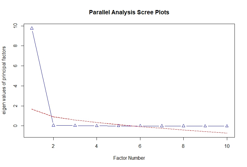 |
| Scree Plot for Number of Factors |
Performing EFA
Here, we extract 3 factors with Varimax rotation using principal axis factoring:
efa_result <- fa(physio_data, nfactors = 3, rotate = "varimax", fm = "pa")
Interpreting Factor Loadings
Print and interpret loadings:
print(efa_result)
Image: Factor Loadings Table (cutoff = 0.3)
print(efa_result$loadings, cutoff = 0.3)
Visualizing the Results
Create a factor diagram to illustrate the relationships:
fa.diagram(efa_result)
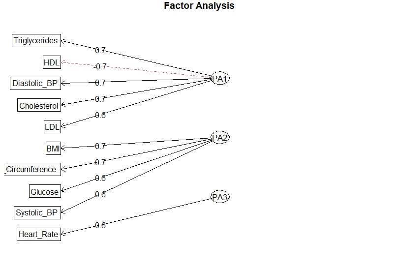 |
| Factor Diagram |