Mastering CFA for Plant Stress Indicators Using R Studio
Confirmatory Factor Analysis (CFA) is a powerful multivariate statistical technique that allows researchers to test hypotheses about the relationships between observed variables and underlying latent constructs. In this tutorial, we will walk you through how to perform CFA in R using plant stress indicators as an example. This post includes detailed R code, visual outputs, and explanations that will guide both beginners and experienced users in structural equation modeling (SEM).
1. What is Confirmatory Factor Analysis (CFA)?
Confirmatory Factor Analysis is a technique used to test whether a hypothesized relationship between observed variables and their underlying latent variables holds true. Unlike Exploratory Factor Analysis (EFA), CFA is theory-driven—meaning you specify the structure beforehand and test how well the data fits this structure.
In our case, we hypothesize that plant stress responses can be categorized into two latent constructs:
- Physiological Stress (PhysStress)
- Biochemical Stress (BioStress)
2. Why Use CFA in Biostatistics?
CFA is widely used in biological and agricultural sciences to validate measurement models where multiple indicators represent a smaller number of latent biological constructs. For example:
- Measuring plant stress responses using traits like chlorophyll content and proline accumulation.
- Understanding latent syndromes in ecology or medicine.
- Testing hypotheses based on theoretical frameworks in physiological research.
3. Tools Required in R for CFA
To begin, we install and load the necessary R packages:
install.packages("lavaan")
install.packages("semPlot")
install.packages("corrplot")
library(lavaan)
library(semPlot)
library(corrplot)
- lavaan is the primary package for running CFA models.
- semPlot is used to create visual path diagrams.
- corrplot helps in generating heatmaps for correlation matrices.
4. Loading and Standardizing the Dataset
We use a synthetic dataset named PlantStressData that contains six variables (30 observations) representing different physiological and biochemical stress indicators in plants.
Physiological Indicators:
- Chlorophyll_Content
- Stomatal_Conductance
- Leaf_Area
Biochemical Indicators:
- Proline_Content
- Antioxidant_Activity
- Lipid_Peroxidation
5. Defining the CFA Model
Next, we define the CFA model with two latent factors:
model <- '
PhysStress =~ Chlorophyll_Content + Stomatal_Conductance + Leaf_Area
BioStress =~ Proline_Content + Antioxidant_Activity + Lipid_Peroxidation
'
- PhysStress is hypothesized to explain variation in the physiological indicators.
- BioStress is hypothesized to explain variation in the biochemical indicators.
6. Fitting the CFA Model
Using the cfa() function from the lavaan package, we fit the model to our standardized data:
fit <- cfa(model, data = PlantStressData_scaled)
7. Evaluating Model Fit
To assess whether the model fits the data well, we generate a summary with fit indices:
summary(fit, fit.measures = TRUE, standardized = TRUE)
Key Fit Indices:
- Chi-square Test: Lower values with high p-values indicate a good fit.
- CFI (Comparative Fit Index): >0.90 is acceptable; >0.95 is excellent.
- RMSEA (Root Mean Square Error of Approximation): <0.08 is acceptable.
- SRMR (Standardized Root Mean Square Residual): <0.08 is good.
standardized = TRUE argument shows the standardized factor loadings, which are easier to interpret.8. Drawing the Path Diagram
To visualize the relationships between latent and observed variables, we use semPaths():
semPaths(fit,
what = "std",
whatLabels = "std",
layout = "tree",
edge.label.cex = 1.1,
sizeMan = 12,
sizeLat = 8,
title = FALSE,
nCharNodes = 0)
This graphically displays:
- Latent variables as circles
- Observed variables as rectangles
- Standardized factor loadings on the connecting arrows
 |
| Path Diagram |
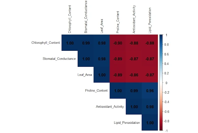
9. Visualizing the Correlation Heatmap
Before or after CFA, it's insightful to examine how variables are interrelated using a correlation heatmap:
cor_matrix <- cor(PlantStressData)
print(cor_matrix)
corrplot(cor_matrix,
method = "color",
type = "upper",
addCoef.col = "black",
tl.col = "black",
tl.cex = 0.8)
This plot highlights:
- Positive and negative correlations
- Strength of relationships
- Potential multicollinearity
 |
| Correlation Heatmap |
10. Interpretation and Practical Applications
The standardized loadings in the CFA output tell us how strongly each observed variable is related to its latent construct. For example:
- A high loading of Chlorophyll_Content on PhysStress suggests it's a good indicator of physiological stress.
- Similarly, a strong loading of Proline_Content on BioStress supports its role in biochemical stress response.
Applications:
- Agricultural Research: Identify stress-resilient plant varieties.
- Ecological Monitoring: Evaluate environmental stressors on vegetation.
- Medical/Biological Sciences: Validate latent traits (e.g., immune response indicators).
CFA provides a statistically valid framework for such multi-dimensional analyses.
11. Final Thoughts
Confirmatory Factor Analysis (CFA) is not just a statistical technique—it’s a bridge between theory and data. With R’s powerful packages like lavaan, semPlot, and corrplot, researchers can validate models with precision and clarity.
This tutorial has taken you through every major step:
- Loading and cleaning data
- Hypothesis specification
- Model fitting
- Visualization and interpretation
Takeaway Line:
"Use Confirmatory Factor Analysis in R Studio to validate plant stress indicators and visualize latent structures using CFA path diagrams and correlation heatmaps for accurate biological interpretation."
Optimize Your CFA Workflow in R Today!
If you're a biostatistician, ecologist, or life science researcher, mastering CFA in R can significantly improve the accuracy and impact of your work. Bookmark this guide or share it with your research team for future reference.