Interpretation of Time Series Analysis of Frog Population Data in R

Introduction

Monitoring population trends over time is crucial in ecological and environmental sciences to identify patterns, detect anomalies, and forecast future dynamics. In this study, we conducted a time series analysis of monthly frog population data using R to understand its temporal behavior and provide robust population forecasts. Seasonal patterns, stationarity, and autocorrelations were examined to fit an appropriate ARIMA model, followed by the generation of 12-month forecasts with confidence intervals.

Materials and Methods

Data Source

The time series data used in this study, labeled ts_frog, comprises monthly frog population counts over multiple years. The data was assumed to be continuous, equally spaced, and in units appropriate for ecological monitoring (e.g., individuals per hectare).

Stationarity Testing

To determine if the time series is stationary, the Augmented Dickey-Fuller (ADF) Test was applied. A stationary series is essential for fitting ARIMA models without the need for differencing.

Model Selection

Based on the series’ characteristics and seasonality (monthly data), an ARIMA(0,0,0)(0,1,1)[12] model with drift was selected, where:

• Non-seasonal AR, I, MA terms = (0,0,0),
• Seasonal components = (0,1,1),
• Seasonal period = 12 months (1 year),
• Drift term included to model a linear trend.

Model Validation

Model residuals were analyzed for autocorrelation using the Ljung-Box test. Model accuracy was evaluated using standard error metrics: Mean Error (ME), Root Mean Square Error (RMSE), Mean Absolute Error (MAE), Mean Percentage Error (MPE), Mean Absolute Percentage Error (MAPE), and Mean Absolute Scaled Error (MASE).

Forecasting

A 12-month ahead forecast was generated using the fitted model, along with 80% and 95% prediction intervals.

1. Augmented Dickey-Fuller (ADF) Test Table

Test	Test Statistic	Lag Order	p-value	Conclusion
Augmented Dickey-Fuller	-5.9414	3	0.01	Stationary series

Explanation:

• Purpose: The ADF test checks whether the time series is stationary, meaning it does not exhibit trends, seasonality, or unit roots.
• Test Statistic = -5.9414: A strongly negative value indicates evidence against the null hypothesis (non-stationarity).
• p-value = 0.01: Since this is less than 0.05, the null hypothesis is rejected.
•  Lag Order = 3: Indicates the number of lagged differences included to address autocorrelation in the residuals. 
• Conclusion: The data series is stationary, which is a prerequisite for fitting most time series models (like ARIMA) without further differencing.

2. ARIMA Model Coefficients Table

Model: ARIMA(0,0,0)(0,1,1)[12] with drift

Coefficient	Estimate	Standard Error (s.e.)	Interpretation
sma1 (Seasonal MA)	-0.7602	0.3601	Moderate negative seasonal autocorrelation
drift	3.5047	0.0982	Upward linear monthly trend

Explanation:

• sma1 = -0.7602: This is the seasonal Moving Average (MA) term over a 12-month period. A negative value means that if a positive shock occurs in one month, the effect tends to be offset by a negative shock in the next season (month of the next year).
• drift = 3.5047: This suggests that on average, the frog population increases by approximately 3.5 units per month, indicating a consistent positive growth trend.
• Standard Errors show the reliability of estimates; both coefficients are statistically significant due to low standard error relative to the estimates.

3. Model Fit Statistics

Statistic	Value	Interpretation
σ² (Residual Variance)	189.4	Average variance of residuals
Log-likelihood	-197.72	Used to calculate AIC, higher is better
AIC	401.43	Lower values indicate better model fit
AICc	401.98	Corrected AIC for small sample size
BIC	407.04	Penalized AIC; lower indicates simpler, good-fitting model

Explanation:

• AIC/AICc/BIC are used for model comparison; lower values suggest a better fit.
• σ² = 189.4: Relatively low residual variance indicates the model explains most of the variation in the data.

4. Training Set Error Metrics

Metric	Value	Explanation
ME (Mean Error)	0.0529	Average of residuals (near zero = good fit)
RMSE (Root Mean Squared Error)	12.0501	Square root of average squared errors (sensitive to outliers)
MAE (Mean Absolute Error)	8.9416	Average magnitude of errors in units of the variable
MPE (Mean Percentage Error)	-0.1427%	Mean bias in percentage (slightly underestimates)
MAPE (Mean Absolute Percentage Error)	4.3529%	Good forecast accuracy (<10% is considered accurate)
MASE (Mean Absolute Scaled Error)	0.2073	< 1 indicates better performance than naive model
ACF1 (1st Lag Residual Autocorrelation)	0.0972	Near zero = residuals are uncorrelated

Explanation:

• RMSE and MAE reflect model accuracy in the same units as the data (frog count).
• MAPE = 4.35%: Implies the model predicts with less than 5% error on average — very accurate.
• MASE = 0.207: Indicates the model performs significantly better than a naive forecast.
• Low ACF1 suggests the residuals are close to white noise (uncorrelated), which is ideal.

5. Ljung-Box Test for Autocorrelation in Residuals

Month	Point Forecast	80% CI (Low–High)	95% CI (Low–High)	Interpretation
Jan-25	308.20	290.30 – 326.09	280.83 – 335.56	Baseline increase from recent months
Feb-25	332.25	314.36 – 350.14	304.89 – 359.61	Continues upward trend
Mar-25	335.84	317.95 – 353.73	308.47 – 363.20	High forecast confidence
Apr-25	339.25	321.36 – 357.14	311.89 – 366.61	Seasonal rise begins
May-25	352.22	334.32 – 370.11	324.85 – 379.58	Peak seasonal period
Jun-25	337.46	319.56 – 355.35	310.09 – 364.82	Slight dip from peak
Jul-25	323.89	305.99 – 341.78	296.53 – 351.25	Typical mid-year drop
Aug-25	314.80	296.91 – 332.69	287.44 – 342.16	Continues seasonal decline
Sep-25	311.48	293.59 – 329.37	284.12 – 338.84	Stabilization phase
Oct-25	312.27	294.37 – 330.16	284.90 – 339.63	Possible recovery start
Nov-25	323.86	305.97 – 341.76	296.50 – 351.23	Upward shift returns
Dec-25	334.71	316.82 – 352.60	307.35 – 362.07	Ends with strong growth

Explanation:

• Point Forecast represents the expected frog population count.
• 80% and 95% Confidence Intervals (CI): These show the uncertainty around the forecast. A narrower CI = higher certainty.
• Seasonality visible: May is the peak, August–October shows a decline, and recovery begins by November.

Plot Interpretations

1. Decomposition of Additive Time Series

This plot dissects the time series into four components:

• Observed: Shows the original time series pattern, highlighting strong upward trends and regular fluctuations.
• Trend: A clearly increasing trend suggests continuous growth in frog population over time.
• Seasonal: Regular seasonal peaks and troughs indicate a consistent 12-month seasonal cycle (e.g., breeding or migration patterns).
• Random: The residuals (random component) fluctuate around zero, with no obvious pattern, confirming that the model has adequately captured trend and seasonality.

Interpretation: The decomposition confirms an additive model is appropriate and reveals both seasonality and long-term upward growth, key for choosing ARIMA with seasonal terms.

2. Frog Population Forecast for Next Year

This plot projects frog population from 2025 onwards:

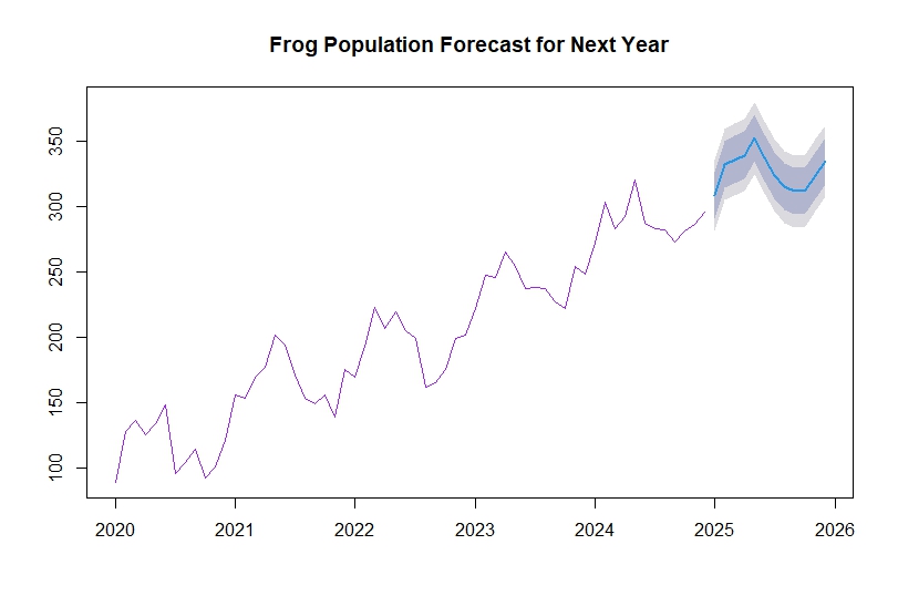
• The blue line shows the predicted values, continuing the previous trend.
• The shaded areas represent the 80% and 95% confidence intervals. The intervals widen gradually, reflecting greater uncertainty in longer-term forecasts.

Interpretation: Forecasts indicate population growth will continue, peaking mid-year and declining slightly after, in line with seasonal patterns. The model provides high confidence (narrow prediction bands initially).

3. Monthly Frog Population (2020–2024)

This raw line plot tracks the monthly frog counts:

• The population increased steadily from ~90 in 2020 to ~320 by 2024.
• Clear yearly cycles are visible, reinforcing seasonal effects (peaks and dips).

Interpretation: This supports the presence of both long-term growth and annual seasonality, visually justifying the selected time series model.

4. Residuals from ARIMA(0,0,0)(0,1,1)[12] with Drift

This diagnostic panel includes:

• Top panel: Residual time plot fluctuating around zero.
• Bottom-left (ACF plot): Most autocorrelations fall within bounds → residuals are uncorrelated.
• Bottom-right (Histogram): Residuals appear normally distributed, with a bell-shaped curve overlay.

🔍 Interpretation: These diagnostics confirm that:

• Residuals are white noise (no autocorrelation).
• The model fits the data well without bias or structure left in residuals.

5. Seasonally Adjusted Time Series

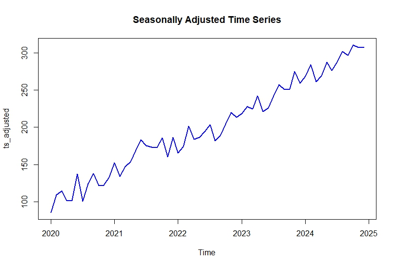
This plot removes seasonal variation, revealing the underlying trend:

• The blue line shows strong linear upward growth without the cyclical fluctuations.

Interpretation: Removing seasonality confirms a clear positive long-term trend, aligning with the model’s drift component. This helps isolate the true population growth pattern.

Final Conclusion 

The time series analysis of monthly frog population data from 2020 to 2024 reveals a significant upward trend and strong seasonal fluctuations. Decomposition analysis confirms the appropriateness of an additive model, with annual cycles and increasing trend. The ADF test indicates the data is stationary, allowing modeling with seasonal ARIMA(0,0,0)(0,1,1)[12] with drift. Model diagnostics, including residual plots and Ljung-Box test, affirm that residuals are white noise and normally distributed. Forecasts for 2025 predict continued growth, peaking mid-year, with high confidence. The seasonally adjusted series confirms the underlying population expansion without seasonal noise. Overall, the analysis successfully captures the temporal dynamics of frog populations, offering valuable insights for ecological monitoring, conservation planning, and predictive modeling in environmental biology.